Tutorial: How to Interpret Grad-CAM Results for FoodDX Models
This tutorial gives a brief introduction and intuition of the Grad-CAM computations and explains how the results from performing Grad-CAM on the Food-Non-Food (FNF) and Food Scoring (FS) models can be used to explain the models themselves.
Outline:
It might be helpful to review the original Grad-CAM paper alongside this tutorial to better understand the computations that Grad-CAM performs.
Brief Overview of Grad-CAM
Grad-CAM stands for Gradient-weighted Class Activation Mapping. It is a popular technique for visualising where a convolutional neural network (CNN) is “looking” when making a prediction.
The explanation that Grad-CAM provides comes in a form of a heatmap, as shown below:
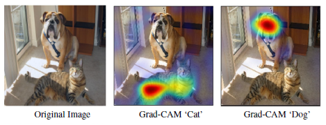
Image taken from original Grad-CAM paper.
Without going too much into the details, here is a list of characteristics of Grad-CAM:
Grad-CAM is class-specific:
It can produce a separate visualisation for every class present in the image.
Grad-CAM is generally used for explaining CNNs used for classification:
As implied from Grad-CAM being class specific, it is good to note that Grad-CAM is generally used for to explain classification (Food-Non-Food model in FoodDX). However, it can be adapted to explain regression applications too (Food Scoring model in FoodDX).
Grad-CAM is a form of post-hoc attention:
It is a method for producing heatmaps to already-trained neural networks with parameters that are already fixed.
Grad-CAM works only on CNNs:
The heatmap that Grad-CAM produces originates from the activation maps from convolutional layers of a CNN (hence it needs CNNs, not a typical vanilla neural network).
That being said, Grad-CAM is generalisable in a sense that it can work on any CNN architecture (as opposed to CAM, which requires a specific kind of CNN architecture).
Understanding the Grad-CAM Computations
To understand how we know where the model is looking, we have to understand what Grad-CAM does under the hood.
As the name implies, Grad-CAM is a series of computations involving the gradients of a given CNN (and a given input) together with a chosen activation map of the model. The result from this series of computations then provides an explanation for the model’s predicted output for a given input image.
This is the series of computations that Grad-CAM performs for a given image, for a given already-trained CNN:
Forward pass the image through the already-trained CNN to get the predictions for every class.
Compute the gradients of the target output class with respect to the pixels of the activation maps from the chosen convolutional layer.
Global average pool the gradients along the channel dimension. This results in each channel of the activation map having its own corresponding globally-average-pooled gradient.
Using the globally-average-pool gradients as weights, do a weighted-sum of the activation maps along the channel dimension. This results in a final single-channel heatmap that has the same width and height of the activation maps.
[OPTIONAL STEP] Apply the ReLU function to the final heatmap to keep only the positive values.
The diagram below is a visual summary of the computations covered above:
How to Interpret Grad-CAM Outputs for FNF and FS FoodDX Models
The Food-Non-Food (FNF) model performs binary classification while the Food Scoring (FS) model performs a regression task. As such, the interpretation of the Grad-CAM heatmaps are slightly different for each model.
1. Explaining the FNF model
The Grad-CAM heatmap produced from the FNF model (and a given input image) can be used to answer the following 2 questions:
Where was the FNF model looking at when it predicted that this image is food / non-food?
Why did the FNF model incorrectly predict this image as food (or non-food)?
1.1. The 2 rules for interpreting Grad-CAM results for FNF model
The 2 general rules to keep in mind when interpreting the Grad-CAM results for the FNF model are:
Positive (green) regions contain features that have a positive influence on the class of interest.
Negative (red) regions contain features that have a negatvie influence on the class of interest.
i.e. These red regions contain features that have positive influence on the rest of the classes (apart from the class of interest).
In the case of the FNF model, the class of interest is an image’s ground truth class. i.e. If an image is food, its class of interest is the food class (and vice versa).
Below, we use 2 example Grad-CAM results to better exemplify the explanations that we can get from the Grad-CAM heatmaps.
1.2. Example 1: Correct classification
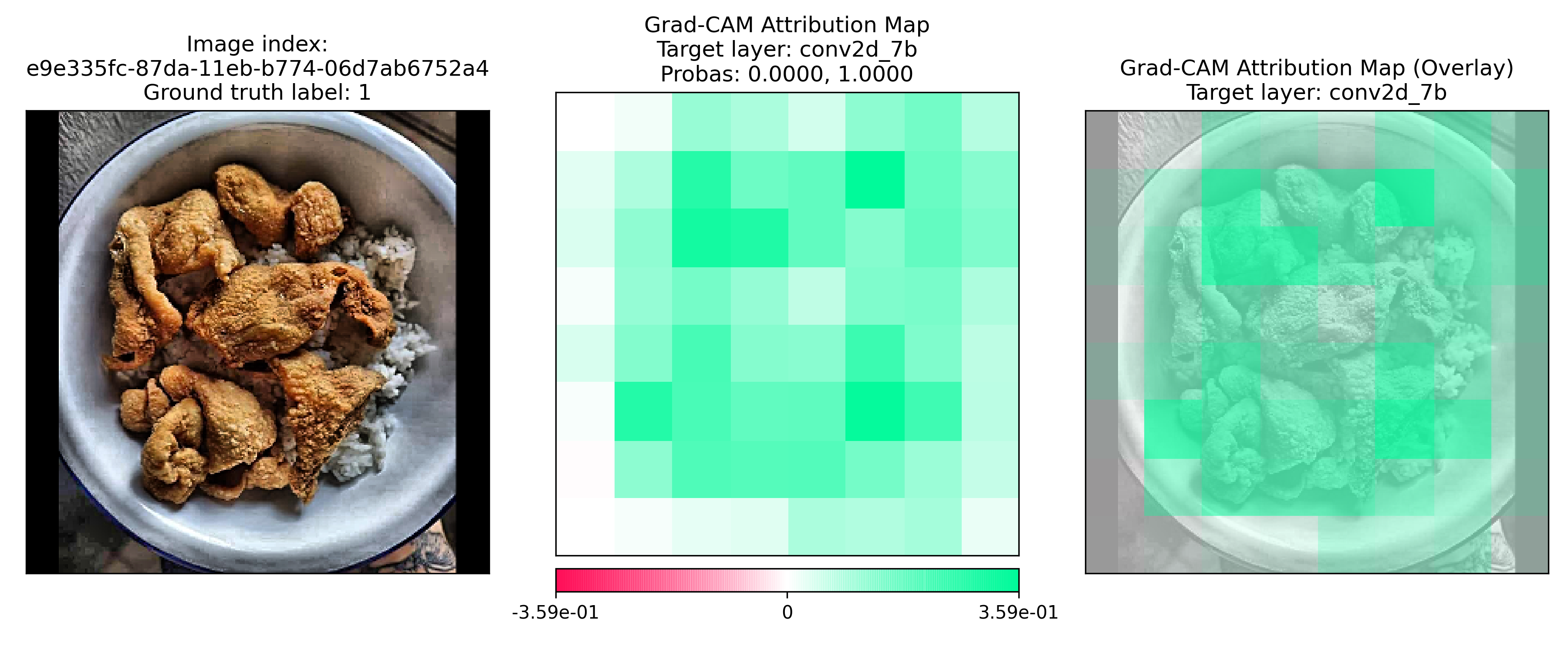
The image above is predicted perfectly as food, with a predicted probability for non-food = 0.0 and predicted probability for food = 1.0. In this case, it is appropriate to ask Question 1, “Where was the FNF model looking at when it predicted that this image is food?”
The positive (green) areas are where the FNF model looked at when it predicted a probability of 1.0 for food. These green regions are regions that contain features that are highly activated in the model during the forward pass (prediction) and hence have a positive influence on the predicted probability for the food class. Here, we see that the FNF model is clearly looking at the food in the bowl (as opposed to the background, bowl, etc.) when making a prediction for the food class.
Furthermore, there are almost no negative (red) regions, showing that to the FNF model, there is almost nothing in the image that suggests this image might be non-food.
1.3. Example 2: Wrong classification
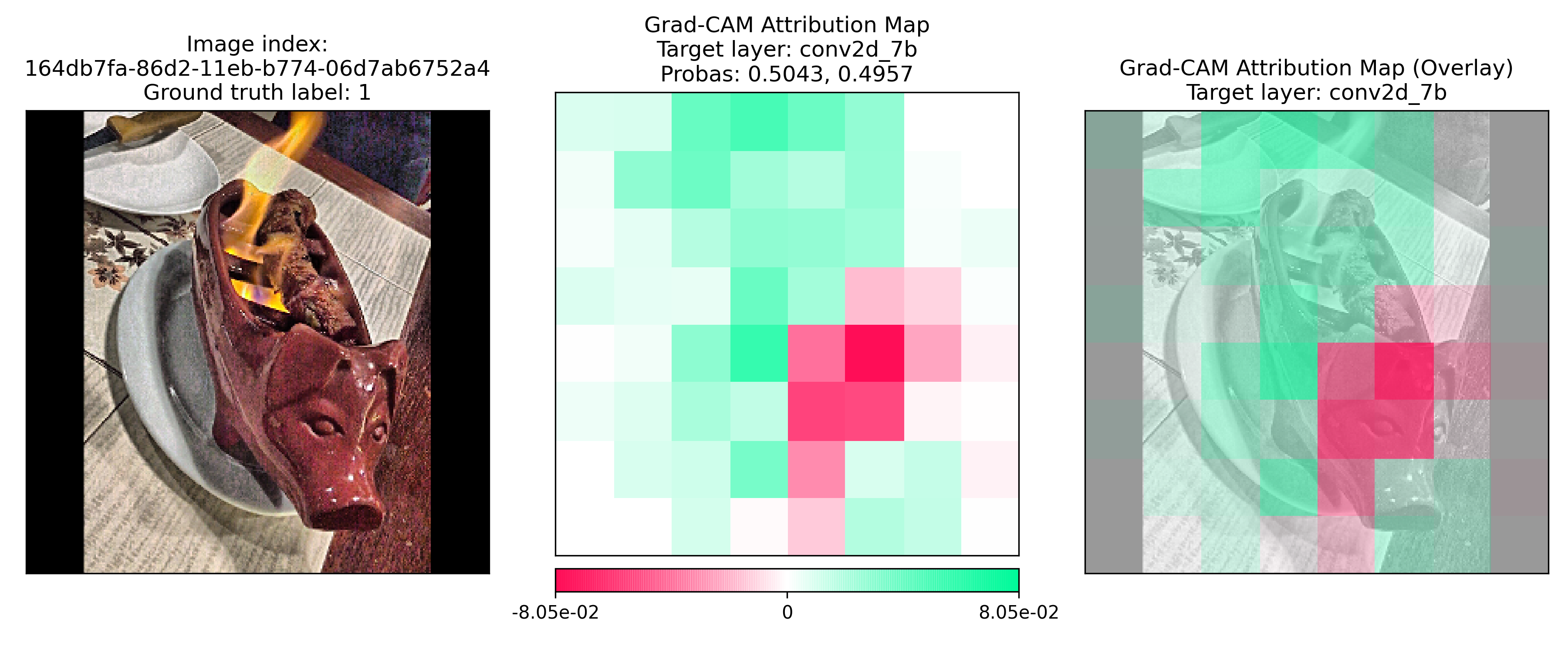
This is a case of the FNF model making a wrong prediction. The FNF model predicted this image as non-food when it is in fact a food dish (predicted probability for non-food = 0.5043, predicted proability for food = 0.4957). In this case, it is appropriate to ask Question 2, “Why did the FNF model incorrectly predict this image as non-food?”
As with Exmaple 1 above, the green regions are regions that have a positive influence on the food class prediction. These regions are quite spread out across the actual dish and the background, showing that the model was not able to focus entirely on the food (as opposed to how it was able to focus on the food in Exmaple 1).
However, more importantly, there are negative (red) regions highlighting the face of the pig (serving dish). This face is a feature that has a strong negative influence on the food class prediction. The FNF model was looking at this face and classifying this image as non-food instead of food.
2. Explaining the FS model
The plotted Grad-CAM results for the FS model differ slightly from those from
the FNF model. There are 4 columns of Grad-CAM heatmaps in each plot, each for
model 1, 2, 3 and the average model. You can refer to the documentation for
XAI.utils.plot_helpers.fs_plot() for more details.
Similar to using Grad-CAM to explain the FNF model, the Grad-CAM heatmap can be used to answer the following fundamental question for the FS model:
Which area(s) contributed positively / negatively to the predicted food score?
That is the fundamental question of interest because most other questions that explores explaining the FS model’s predictions can be broken back down to that question. For exmaple, “Why did the model under-predict the food score (i.e. predicted food score is lower than the ground truth)?” ➔ “Where was the model looking at when it made the low prediction?” ➔ “Which area(s) contributed negatively (and positively) to the food score?”
2.1. The 2 rules for interpreting Grad-CAM results for FS model
The two general rules to keep in mind when interpreting the Grad-CAM results for the FS model are:
Positive (green) regions contain features that have a positive influence on the predicted food score.
There are 2 ways to think about this:
If these regions in the image are enhanced, we should expect the FS model to predict a higher food score.
If these regions are removed from the image, we should expect the FS model to predict a lower food score.
Negative (red) regions contain features that have a positive influence on the predicted food score.
The mental framework to think about this is the opposite of the above:
If these regions in the image are enhanced, we should expect the FS model to predict a lower food score.
If these regions are removed from the image, we should expect the FS model to predict a higher food score.
2.2. Example 1: FS model under-predicting food score
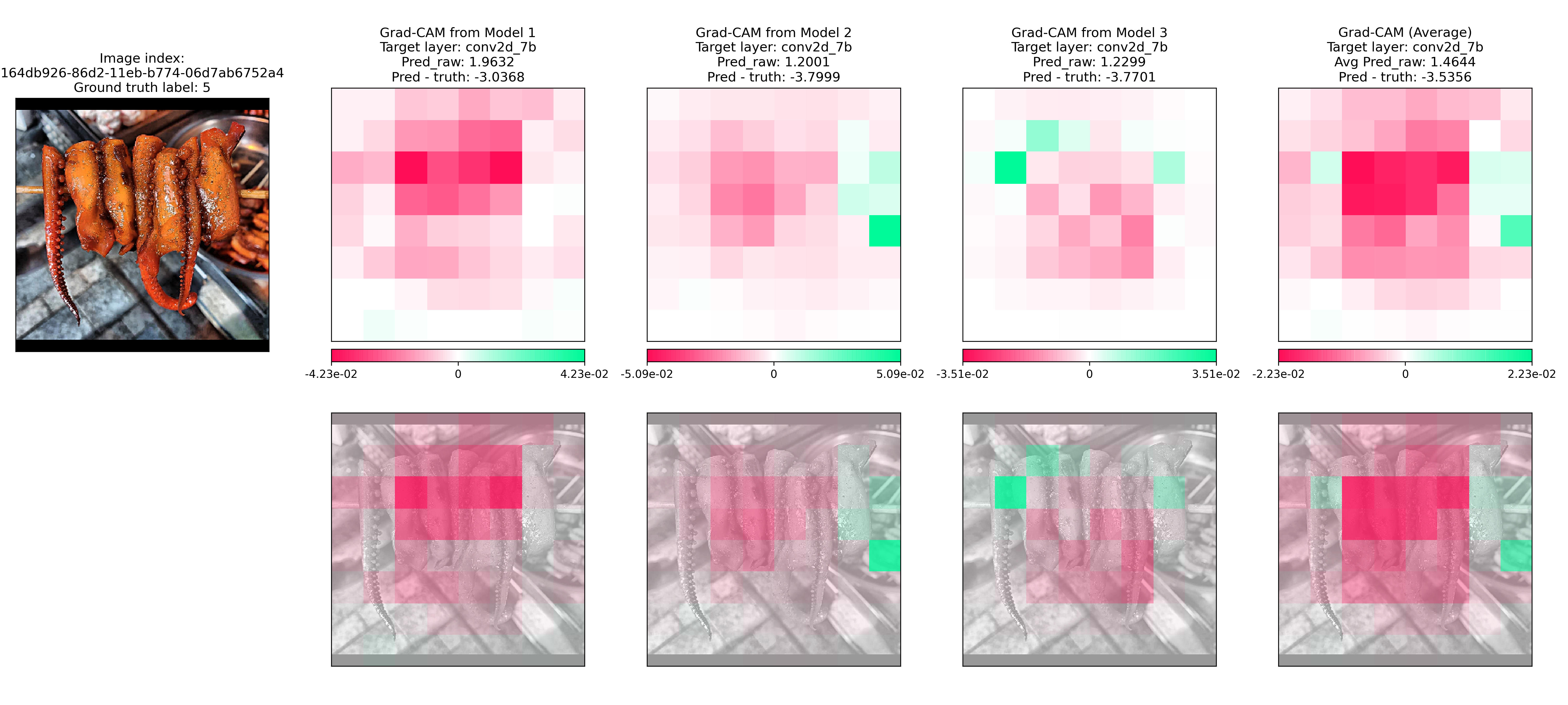
In this example, the average FS model predicted a food score of 1 when the ground truth food score is a 5 (i.e. under-prediction). In the Grad-CAM heatmap, the red regions contain features that brought the food score down and hence caused the under-prediction. We can see that the FS model is correctly looking at the food (as opposed to elsewhere) but yet it is inaccurately predicting its food score.
2.3. Example 2: FS model over-predicting food score
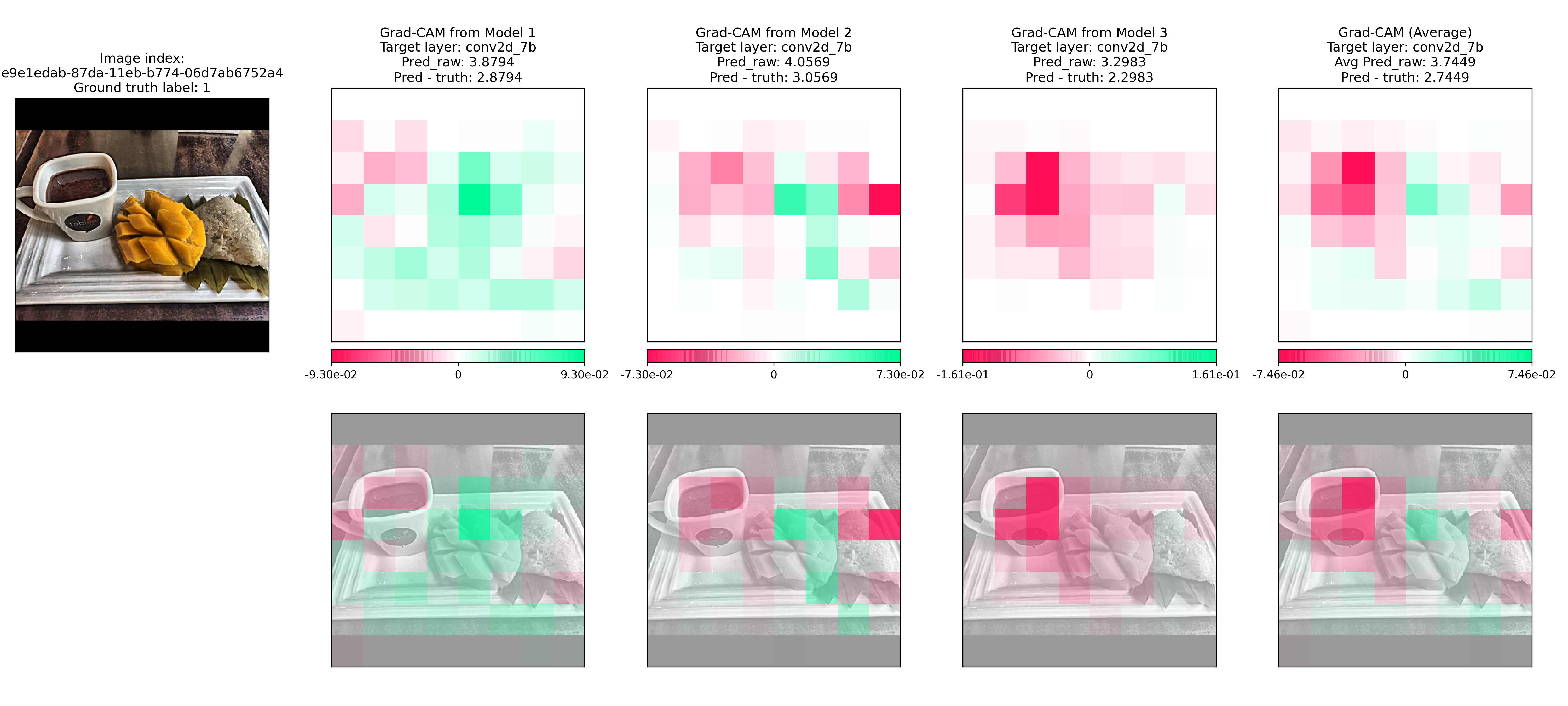
In this example, the average FS model predicted a food score of 4 when the ground truth food score is a 1 (i.e. over-prediction). In the Grad-CAM heatmap, we see regions of red and green. The green regions were responsible for bringing the predicted food score up. This means that the mangoes (covered in green) were what caused the over-prediction.
2.4. Limitations of Grad-CAM’s explanation for explaining the FS model
While we see that the Grad-CAM heatmap can tell us which areas of the image contributed to the over (or under) predicted food score, it cannot tell us exactly why the food score is the value that it is.
For example, the heatmap can give us an explanation on why there was an over-prediction. This explanation comes from showing us where the FS model looked at when it predicted a food score of 5 when the ground truth score is 1. However, the heatmap cannot tell us exactly why the over-prediction was a 5 instead of a 4. There is a distinction between those two explanations.