Tutorial: Doing Grad-CAM on the Food Scoring (FS) model
This is a tutorial on how to perform Grad-CAM on the FS model using the
XAI.FSGradCAM() class that is provided in this library.
Summary of the recommended workflow:
Instantiate the 3 desired FS model and load their desired pretrained weights.
Create a PyTorch dataset using the
XAI.utils.datasets.DatasetFromCSV()class.Instantiate the
XAI.FSGradCAM()object.Do the Grad-CAM algorithm on the dataset created in Step 2 using the
do_gradcam()function.If necessary, plot and save the Grad-CAM results using the
plot_gradcam()function.
There will be 2 ways that you can perform thm Grad-CAM on the FS model, both of which will be covered in this tutorial:
To begin, activate the virtual environment that has the XAI library
installed and import the library.
1 | import XAI
|
Method 1: Using the imported XAI library
Step 1: Load the 3 desired PyTorch models
This tutorial assumes that this step is already completed and that the 3 desired
PyTorch models are loaded into the variables model_1, model_2 and
model_3. Refer to this tutorial if necessary.
Step 2: Creating the dataset
This tutorial assumes that this step is already completed and that the dataset
of images is created as the ds variable. Refer to
Tutorial: Creating a DatasetFromCSV Dataset for a walkthrough on how to create the dataset.
The dataset ds used in this tutorial contains 10 images.
Step 3: Instantiate FSGradCAM() class object
Instantiate the XAI.FSGradCAM() class by doing the following. Here, the
target layer used in the Grad-CAM computation is conv2d_7b.
1 2 3 4 5 6 | fs_gc = XAI.FSGradCam(
model_1=model_1,
model_2=model_2,
model_3=model_3,
target_layer_name="conv2d_7b",
)
|
The fs_gc object has the following 3 attributes:
>>> fs_gc.device
device(type='cuda', index=0)
>>> fs_gc.target_layer_name
'conv2d_7b'
>>> fs_gc.models_list
# This print a list of tuples as such:
# [(model_1.eval().to(self.device), target_layer_list[0]),
#  (model_2.eval().to(self.device), target_layer_list[1]),
#  (model_3.eval().to(self.device), target_layer_list[2])]
Step 4: Do the Grad-CAM using the do_gradcam() function
This function does the following 3 observable things:
Computes the Grad-CAM attribution map for each image and saves each map as a numpy array (
.npyfile) in the specified output folder (output_folder).Returns a Pandas DataFrame containing the results of performing Grad-CAM and saves this DataFrame as
gradcam_metadata.csvinoutput_folder.Plots and saves the Grad-CAM numpy arrays as
.pngfiles ifplot_gradcam=True.
The following folder structure will be created in output_folder to save the
3 outputs listed above:
output_folder/
├── gradcam_metadata.csv
│
├── gradcam_numpy_arrays/
│   ├── 164c728e-86d2-11eb-b774-06d7ab6752a4.npy
│   ├── 164c728f-86d2-11eb-b774-06d7ab6752a4.npy
│   ├── ...
│   └── 164c72a5-86d2-11eb-b774-06d7ab6752a4.npy
│
└── gradcam_plots/ <--- This folder will be created if `plot_gradcam=True`
    ├── 164c728e-86d2-11eb-b774-06d7ab6752a4.png
    ├── 164c728f-86d2-11eb-b774-06d7ab6752a4.png
    ├── ...
    └── 164c72a5-86d2-11eb-b774-06d7ab6752a4.png
Note:
The dataset passed into the function is
ds.The function performs Grad-CAM on batches of images of size
batch_size.The ReLU function can be included or excluded in the Grad-CAM computation by setting
relu_attributionsto eitherTrueorFalserespectively. Refer to Tutorial: How to Interpret Grad-CAM Results for FoodDX Models to understand the purpose of the ReLU function. It is recommended to set this as ``False``.If
return_metadata=True, each batch of images will be forward-passed into the model to get the model’s predicted probabilities for each image. These probabilities will be included in the returned DataFrame.
You can refer to the documentation on the FSGradCAM.do_gradcam() function
for an explanation of each argument.
1 2 3 4 5 6 7 8 | fs_results_df = fs_gc.do_gradcam(
image_dataset=ds,
batch_size=2,
relu_attributions=False,
return_metadata=True,
output_folder="/output_folder",
plot_gradcam=False
)
|
# Output:
Working on batch 1 of 5, batch_size = 2, model 1...
Computing metadata for model 1...
Working on batch 1 of 5, batch_size = 2, model 2...
Computing metadata for model 2...
Working on batch 1 of 5, batch_size = 2, model 3...
Computing metadata for model 3...
Computing metadata for average model...
Working on batch 2 of 5, batch_size = 2, model 1...
Computing metadata for model 1...
Working on batch 2 of 5, batch_size = 2, model 2...
Computing metadata for model 2...
Working on batch 2 of 5, batch_size = 2, model 3...
Computing metadata for model 3...
Computing metadata for average model...
Working on batch 3 of 5, batch_size = 2, model 1...
Computing metadata for model 1...
Working on batch 3 of 5, batch_size = 2, model 2...
Computing metadata for model 2...
Working on batch 3 of 5, batch_size = 2, model 3...
Computing metadata for model 3...
Computing metadata for average model...
Working on batch 4 of 5, batch_size = 2, model 1...
Computing metadata for model 1...
Working on batch 4 of 5, batch_size = 2, model 2...
Computing metadata for model 2...
Working on batch 4 of 5, batch_size = 2, model 3...
Computing metadata for model 3...
Computing metadata for average model...
Working on batch 5 of 5, batch_size = 2, model 1...
Computing metadata for model 1...
Working on batch 5 of 5, batch_size = 2, model 2...
Computing metadata for model 2...
Working on batch 5 of 5, batch_size = 2, model 3...
Computing metadata for model 3...
Computing metadata for average model...
Notice that the do_gradcam() function loops through the batches of images
and the 3 models using the following logic:
1 2 3 4 5 6 7 8 9 | ╔═════════════╗
║ Pseudo-code ║
╚═════════════╝
for batch in batches:
for model in models:
perform Grad-CAM computation for this model
perform metadata computation for this model (if return_metadata=True)
if model == model_3:
perform metadata computation for average model (if return_metadata=True)
|
The returned DataFrame (fs_results_df) will look like the following:
>>> fs_results_df
id |
target_layer |
food_score |
path_fns |
path_gradcam |
path_gradcam_plot |
m1_pred |
m1_diff |
m2_pred |
m2_diff |
m3_pred |
m3_diff |
avg_pred_raw |
avg_pred_clip |
avg_diff_raw |
avg_diff_clip |
|---|---|---|---|---|---|---|---|---|---|---|---|---|---|---|---|
164c729b-86d2-11eb-b774-06d7ab6752a4 |
conv2d_7b |
1 |
path/to/original/image/164c729b-86d2-11eb-b774-06d7ab6752a4.png |
output_folder/gradcam_numpy_arrays/164c729b-86d2-11eb-b774-06d7ab6752a4.npy |
NaN |
1.486682 |
0.486682 |
1.148806 |
0.148806 |
1.294668 |
0.294668 |
1.310052 |
1.0 |
0.310052 |
0.0 |
… |
… |
… |
… |
… |
… |
… |
… |
… |
… |
… |
… |
… |
… |
… |
… |
If
return_metadata=False, the following columns will containnanvalues:m1_predm1_diffm2_predm2_diffm3_predm3_diffavg_pred_rawavg_pred_clipavg_diff_rawavg_diff_clip
If
plot_gradcam=True, thepath_gradcam_plotcolumn will be populated with the paths to the plotted.pngimages.
Step 5: Plot Grad-CAM results using plot_gradcam(), if necessary
It is also possible to call the plot_gradcam() function separately to plot
and save the Grad-CAM numpy arrays into .png images. The plot_gradcam()
function takes in the DataFrame returned from the do_gradcam() function,
retrieves the necessary information from the columns of the DataFrame to plot
the images.
At this point, it is important to understand that plotting,
showing (aka printing) and saving the images are independent of each other.
While plot_gradcam() always plots the images, whether or not the
images are shown inline and/or saved as a .png file is dependent on the
savefig and plt_show arguments.
If
savefig=Trueandplt_show=True, the plots will both be shown inline and saved as a.pngfile to the folder specified insavefig_dir.If
savefig=Trueandplt_show=False, the plots will not be shown inline but will be saved as a.pngfile to the folder specified insavefig_dir. Vice versa.If
savefig=Falseandplt_show=False, the plots will not be saved and shown inline. It is expected that this case is unhelpful and will not be used.
The following folder structure will be created in savefig_dir where the
images will be saved. Here, you can see that if the same folder is used for the
do_gradcam() and plot_gradcam() functions, we will end up with the
folder structure that is shown here.
output_folder/
├── gradcam_metadata.csv <--- If `save_csv=True`, this file will be created and saved.
│
└── gradcam_plots/
    ├── 164c728e-86d2-11eb-b774-06d7ab6752a4.png
    ├── 164c728f-86d2-11eb-b774-06d7ab6752a4.png
    ├── ...
    └── 164c72a5-86d2-11eb-b774-06d7ab6752a4.png
You can refer to the documentation on the FSGradCAM.plot_gradcam() fuction
for an explanation of each argument.
1 2 3 4 5 6 7 | fs_results_df = fs_gc.plot_gradcam(
do_gradcam_df=fs_results_df,
savefig_dir="/output_folder",
savefig=True,
plt_show=True,
save_csv=True
)
|
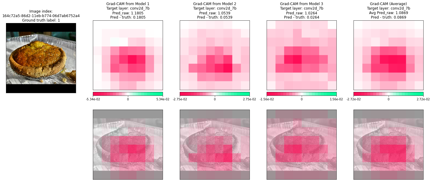
Below is a sample of the output from the plot_gradcam() function that you
should expect to see.
Plotting Grad-CAM results for 164c729b-86d2-11eb-b774-06d7ab6752a4...
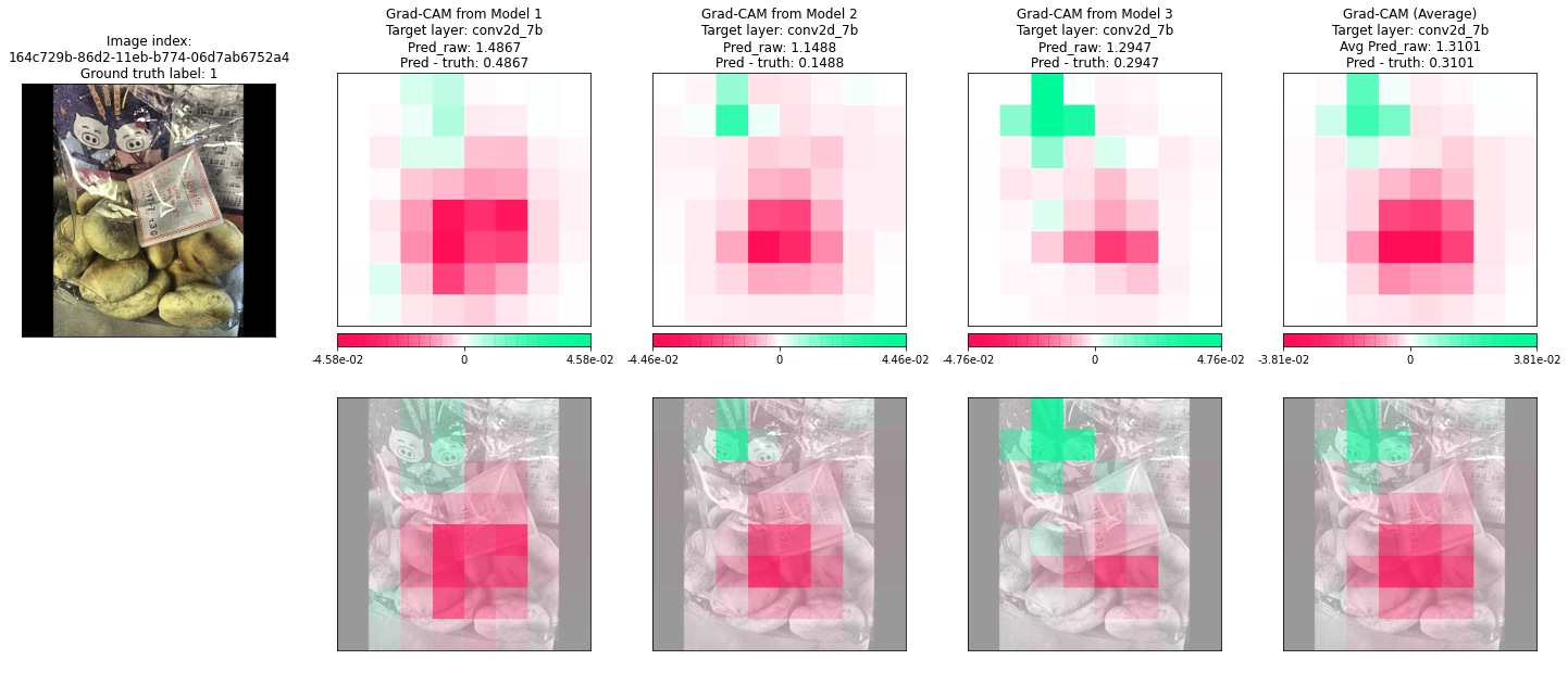
Plotting Grad-CAM results for 164c72a5-86d2-11eb-b774-06d7ab6752a4...
Method 2: Using the Command Line Interface (CLI) Tool
A CLI is the second option that can be used to perform Grad-CAM on the FS
model. Unlike Method 1, the CLI does not
require the user to manually execute
Step 1 and
Step 2 before running the
do_gradcam() and plot_gradcam() functions. This is because the CLI
executes the above 5 steps all together in a single call.
To get an overview of the CLI tool and its arguments, refer to Tutorial: Overview of the Command Line Interface (CLI).
Assuming that we are running the CLI tool from the following parent folder…
.
├── data/
│   ├── data.csv
│   └── images/
│       ├── 164c728e-86d2-11eb-b774-06d7ab6752a4.png
│       ├── 164c728f-86d2-11eb-b774-06d7ab6752a4.png
│       ├── ...
│       └── 164c72a5-86d2-11eb-b774-06d7ab6752a4.png
├── checkpoints/
│   ├── epoch_53.pth
│   ├── epoch_195.pth
│   └── epoch_497.pth
└── otuput_folder/
we will have the following paths to the arguments of the CLI tool:
path_to_csv = ./data/data.csvpretrained_weights_folder = ./checkpoints/epoch_104.pthoutput_folder = ./output_folder
To maintain consistency with Method 1, we will still be:
Using
conv2d_7bas the target layerbatch_size=2relu_attributions=Falsereturn_metadata=Trueplot_gradcam=True
To perform Grad-CAM on the FS model, run the following in the command line:
$ XAI FS ./data/data.csv ./checkpoints ./output_folder conv2d_7b --batch_size 2 --return_metadata --plot_gradcam

  Arguments passed to the parser:
  -------------------------------
  fnf_or_fs : FS
  path_to_csv : .data/data2.csv
  pretrained_weights_folder : ./checkpoints
  output_folder : ./output_folder
  target_layer_name : conv2d_7b
  batch_size : 2
  relu_attributions : False
  return_metadata : True
  plot_gradcam : True

  About the dataset:
  ------------------
  Number of images: 10
  Batch size: 2

  Running the XAI library:
  ------------------------
  Application                : Food-Non-Food (FS)
  Number of model(s) loaded  : 3
  Working on batch 1 of 5, batch_size = 2, model 1...
  Computing metadata for model 1...
  Working on batch 1 of 5, batch_size = 2, model 2...
  Computing metadata for model 2...
  Working on batch 1 of 5, batch_size = 2, model 3...
  Computing metadata for model 3...
  Computing metadata for average model...
  Working on batch 2 of 5, batch_size = 2, model 1...
  Computing metadata for model 1...
  Working on batch 2 of 5, batch_size = 2, model 2...
  Computing metadata for model 2...
  Working on batch 2 of 5, batch_size = 2, model 3...
  Computing metadata for model 3...
  Computing metadata for average model...
  Working on batch 3 of 5, batch_size = 2, model 1...
  Computing metadata for model 1...
  Working on batch 3 of 5, batch_size = 2, model 2...
  Computing metadata for model 2...
  Working on batch 3 of 5, batch_size = 2, model 3...
  Computing metadata for model 3...
  Computing metadata for average model...
  Working on batch 4 of 5, batch_size = 2, model 1...
  Computing metadata for model 1...
  Working on batch 4 of 5, batch_size = 2, model 2...
  Computing metadata for model 2...
  Working on batch 4 of 5, batch_size = 2, model 3...
  Computing metadata for model 3...
  Computing metadata for average model...
  Working on batch 5 of 5, batch_size = 2, model 1...
  Computing metadata for model 1...
  Working on batch 5 of 5, batch_size = 2, model 2...
  Computing metadata for model 2...
  Working on batch 5 of 5, batch_size = 2, model 3...
  Computing metadata for model 3...
  Computing metadata for average model...
  Plotting Grad-CAM results for 164c729b-86d2-11eb-b774-06d7ab6752a4...
  Saving 164c729b-86d2-11eb-b774-06d7ab6752a4 plot to ./output_folder/gradcam_plots/164c729b-86d2-11eb-b774-06d7ab6752a4.png
  Plotting Grad-CAM results for 164c72a5-86d2-11eb-b774-06d7ab6752a4...
  Saving 164c72a5-86d2-11eb-b774-06d7ab6752a4 plot to ./output_folder/gradcam_plots/164c72a5-86d2-11eb-b774-06d7ab6752a4.png
  ...
Similar to Method 1, the Grad-CAM results
will be saved in output_folder as follows:
.
├── data/
│   ├── data.csv
│   └── images/
│       ├── 164c728e-86d2-11eb-b774-06d7ab6752a4.png
│       ├── 164c728f-86d2-11eb-b774-06d7ab6752a4.png
│       ├── ...
│       └── 164c72a5-86d2-11eb-b774-06d7ab6752a4.png
├── checkpoints/
│   ├── epoch_53.pth
│   ├── epoch_195.pth
│   └── epoch_497.pth
└── otuput_folder/
    └── gradcam_metadata.csv
        │
        ├── gradcam_numpy_arrays/
        │   ├── 164c728e-86d2-11eb-b774-06d7ab6752a4.npy
        │   ├── 164c728f-86d2-11eb-b774-06d7ab6752a4.npy
        │   ├── ...
        │   └── 164c72a5-86d2-11eb-b774-06d7ab6752a4.npy
        │
        └── gradcam_plots/
            ├── 164c728e-86d2-11eb-b774-06d7ab6752a4.png
            ├── 164c728f-86d2-11eb-b774-06d7ab6752a4.png
            ├── ...
            └── 164c72a5-86d2-11eb-b774-06d7ab6752a4.png